FMCW Intro - Target speed

You can open this workbook in Google Colab to experiment with mmWrt

Below is an intro to mmWrt for simple targets position and speed estimation based on 2D FFT Range Doppler

The problem

As distance changes over time, how can FMCW radar measure speed ?

The solution

A 2D FFT will allow to measure the speed of the targets

# Install a pip package in the current Jupyter kernel
import sys
from os.path import abspath, basename, join, pardir
import datetime

# hack to handle if running from git cloned folder or stand alone (like Google Colab)
cw = basename(abspath(join(".")))
dp = abspath(join(".",pardir))
if cw=="docs" and basename(dp) == "mmWrt":
    # running from cloned folder
    print("running from git folder, using local path (latest) mmWrt code", dp)
    sys.path.insert(0, dp)
else:
    print("running standalone, need to ensure mmWrt is installed")
    !{sys.executable} -m pip install mmWrt
print(datetime.datetime.now())

running from git folder, using local path (latest) mmWrt code c:\git\mmWrt
2024-05-23 14:24:57.278064

from os.path import abspath, join, pardir
import sys
import matplotlib.pyplot as plt
import matplotlib.cm as cm
from matplotlib import colors
from numpy import where, expand_dims
from numpy import complex_ as complex

# uncomment below if the notebook is launched from project's root folder
# dp = abspath(join(".",pardir))
# sys.path.insert(0, dp)


from mmWrt.Raytracing import rt_points  # noqa: E402
from mmWrt.Scene import Radar, Transmitter, Receiver, Target  # noqa: E402
from mmWrt import RadarSignalProcessing as rsp  # noqa: E402
from mmWrt import __version__ as mmWrt_ver
print(mmWrt_ver)

0.0.6-pre.1

Step by step

Looking at multiple 1D FFT before doing a 2D FFT

from scipy.fft import fft, fft2
c = 3e8

debug_ON = False
test = 0
NC=32
NA=64
fs0 = 1e5
slope0 = 28e10
tic0 = 1.2e-3
radar = Radar(transmitter=Transmitter(bw=0.2e9, slope=slope0,
                                      t_inter_chirp=tic0,
                                      chirps_count=NC),
              receiver=Receiver(fs=fs0, n_adc=NA, max_adc_buffer_size=256,
                                debug=debug_ON), debug=debug_ON)

x1, v1 = 5, 0
target1 = Target(xt=lambda t: v1*t+x1)
x2, v2 = 3, 0.6
target2 = Target(xt=lambda t: v2*t+x2)

targets = [target1, target2]

bb = rt_points(radar, targets, datatype=complex, debug=debug_ON)
print(bb["chirps_count"])
cube = bb["adc_cube"][0,:,0,0,:]
print(cube.shape)
Z_fft2 = abs(fft2(cube))
Data_fft2 = Z_fft2

plt.xlabel("Range")
plt.ylabel("Velocity")
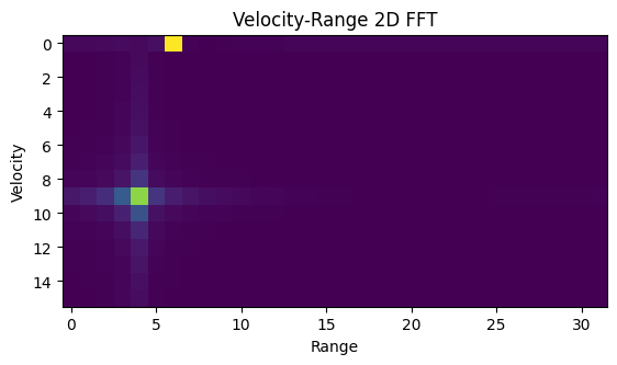
plt.title('Velocity-Range 2D FFT')
plt.imshow(Data_fft2[0:NC//2,:NA//2])

32
(32, 64)

<matplotlib.image.AxesImage at 0x282ae86e010>

Plotting the Range Doppler with units

leveraging the plot_range_doppler utility function

from mmWrt.Plots import plot_range_doppler
fig, _, _ = plot_range_doppler(bb["adc_cube"][0,:,0,0,:], radar, no_speed_shift=False)

# adding comments in picture
fig.text(0.3, 0.5, f"target1: @d={x1}, v={v1}", color="white", fontsize=12)
target1 = plt.Circle((0.22, 0.48), 0.05, fill=False, color="white")
fig.text(0.30, 0.25, f"target2: @d={x2}, v={v2}", color="white", fontsize=12)
target2 = plt.Circle((0.2, 0.25), 0.05, fill=False, color="white")
fig.add_artist(target1)
fig.add_artist(target2)

<matplotlib.patches.Circle at 0x282ae8e5c10>

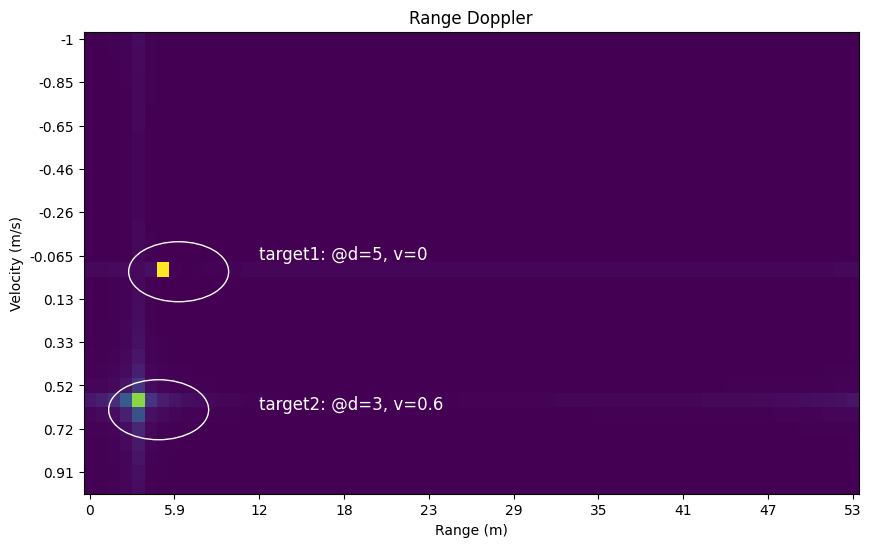
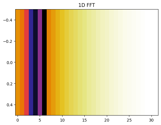
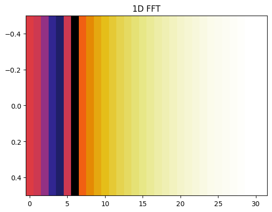
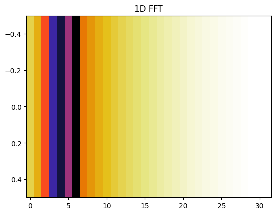
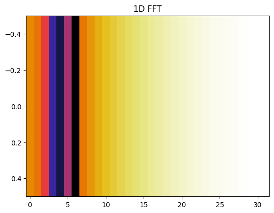
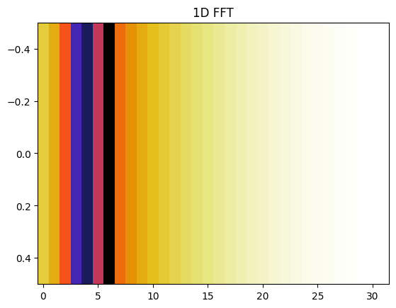
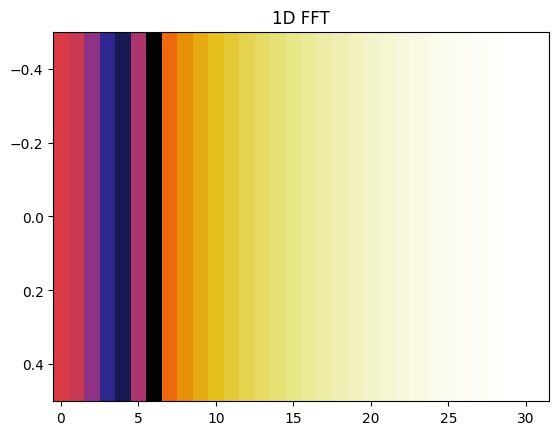
Illustration of 1D FFT and 2D FFT

Plot all the range FFT

Scroll output of next cell to see all the range FFTs

bb = rt_points(radar, targets, debug=debug_ON)
cmap = cm.get_cmap(name='CMRmap_r')
ffts = []
for chirp_i in range(15):
    adc = bb["adc_cube"][0,chirp_i,0,0,:]
    range_profile = fft(adc)

    mag_r = abs(range_profile[:len(range_profile)//2])
    mag_r = expand_dims(mag_r, axis=0)
    plt.imshow(mag_r, cmap,
           aspect='auto',
           norm=colors.LogNorm(vmin=min(mag_r[0][:]), vmax=max(mag_r[0][:])))
    plt.title("1D FFT")
    # plt.savefig(fp_fft_1D)
    plt.show()
    ffts.append(range_profile[:21])

C:\Users\matth\AppData\Local\Temp\ipykernel_8940\2651558762.py:2: MatplotlibDeprecationWarning: The get_cmap function was deprecated in Matplotlib 3.7 and will be removed two minor releases later. Use ``matplotlib.colormaps[name]`` or ``matplotlib.colormaps.get_cmap(obj)`` instead.
  cmap = cm.get_cmap(name='CMRmap_r')

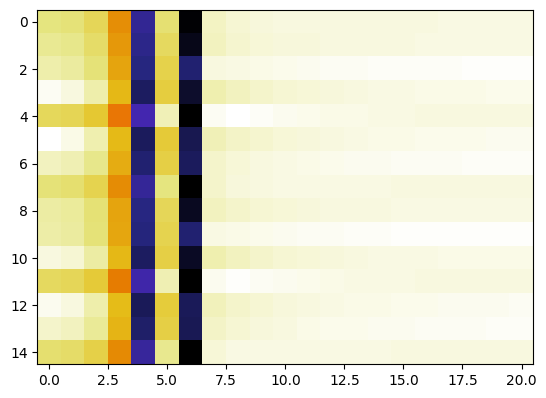
Range FFT on cube

1D FFT on 2D cube, shows 2 targets

from numpy import array
ffts = array(ffts)
plt.imshow(abs(ffts), cmap=cmap)

<matplotlib.image.AxesImage at 0x282ae9709d0>

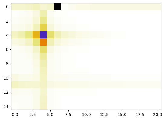
Range Doppler FFT on cube

2nd FFT on 2D cube shows one static target and one moving

similarly as to a 2D FFT would.

fft2 = fft(ffts, axis=0)
plt.imshow(abs(fft2), cmap=cmap)

<matplotlib.image.AxesImage at 0x282aea06850>