FMCW Intro - Grouping

You can open this workbook in Google Colab to experiment with mmWrt

Below is an intro to mmWrt for simple scatterers position estimation

For a generic introduction to mmWave sensors: Watch Here

The problem

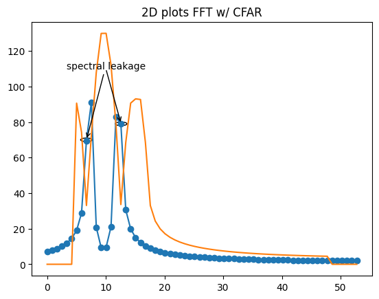
As distance estimation is based on FFT, spectral leakage even after CFAR may lead to detection of too many scatterers.

Changing synthetic scatterer distances in order to make this more visible in the below code

The solution

Pass the index of FFT bin which are over the CFAR threshold to a peak_grouping function which groups them.

Multiple grouping algorithms are possible: * 1D: Adjacent grouping to lead or tail, or interpolation grouping to find the more likely position of the point scatterer

# Install a pip package in the current Jupyter kernel
import sys
from os.path import abspath, basename, join, pardir
import datetime

# hack to handle if running from git cloned folder or stand alone (like Google Colab)
cw = basename(abspath(join(".")))
dp = abspath(join(".",pardir))
if cw=="docs" and basename(dp) == "mmWrt":
    # running from cloned folder
    print("running from git folder, using local path (latest) mmWrt code", dp)
    sys.path.insert(0, dp)
else:
    print("running standalone, need to ensure mmWrt is installed")
    !{sys.executable} -m pip install mmWrt
print(datetime.datetime.now())

running from git folder, using local path (latest) mmWrt code c:\git\mmWrt
2026-07-17 18:40:21.000970

from os.path import abspath, join, pardir
import sys
import matplotlib.pyplot as plt
import matplotlib.cm as cm
from matplotlib import colors
from numpy import where, expand_dims
from numpy import complex128 as complex

from mmWrt.Raytracing import rt_points  # noqa: E402
from mmWrt.Scene import Radar, Transmitter, Receiver, Scatterer  # noqa: E402
from mmWrt import RadarSignalProcessing as rsp  # noqa: E402

Exposing the problem

Without grouping, spectral leakage and guard cells lead to too many scatterers identified

c = 3e8

debug_ON = False
test = 0
chirp_bandwidth = 0.2e9
chirp_slope0 = 70e8
chirp_end_time0 = chirp_bandwidth/chirp_slope0
chirp_period0 = 0.15
radar = Radar(transmitter=Transmitter(chirp_end_time=chirp_end_time0,
                                      chirp_slope=chirp_slope0,
                                      chirp_count=64),
              receiver=Receiver(adc_sample_rate=5e3, adc_sample_count=128, adc_sample_count_max=1024,
                                debug=debug_ON), debug=debug_ON)

scatterer1 = Scatterer(7.2)
scatterer2 = Scatterer(12.1)

scatterers = [scatterer1, scatterer2]

bb = rt_points([radar], scatterers,
               radar, datatype=complex, debug=debug_ON)
Distances, range_profile = rsp.range_fft(bb["adc_cube"][0,0,0,:], bb, debug=debug_ON, full_FFT=False)
mag_r = abs(range_profile)
ca_cfar = rsp.cfar_ca(mag_r, train_cell_count=10,
                      guard_cell_count=1, pfa=1e-1)

mag_c = abs(ca_cfar)
# little hack to remove small FFT ripples : mag_r> 5
scatterer_filter = ((mag_r > mag_c) & (mag_r > 20))

index_peaks = where(scatterer_filter)[0]
# grouped_peaks = rsp.peak_grouping_1d(index_peaks)

found_scatterers = [Scatterer(Distances[i]) for i in index_peaks]
error = rsp.error([scatterer1, scatterer2], found_scatterers)
print("synthetic scatterers", [s.distance() for s in scatterers])
print("found scatterers", [s.distance() for s in found_scatterers])
print("amplitude found scatterers", [mag_r[i] for i in index_peaks])
print("error is", error)

# 2D representation of the FFT and CFAR
# plot on X,Y axis the FFT and CFAR
figure, axes = plt.subplots()
plt.plot(Distances, mag_r, '-o')
plt.plot(Distances, mag_c)
plt.title("2D plots FFT w/ CFAR")

# Add illustration of spectral leakage
# annotate
# xy: position of arrow
# xytext: position of text
xytext = (10, 110)
leak1_xy = (6.7, 70)
leak2_xy = (12.6, 79)

leakage_1 = plt.Circle( leak1_xy, 1, fill=False)
leakage_2 = plt.Circle( leak2_xy, 1, fill=False)
axes.add_artist(leakage_1)
axes.add_artist(leakage_2)

plt.annotate("spectral leakage", xy=leak1_xy,xytext=xytext,
             horizontalalignment="center",
             # Custom arrow
             arrowprops=dict(arrowstyle='->',lw=1)
             )

plt.annotate("", xy=leak2_xy,xytext=xytext,
             horizontalalignment="center",
             # Custom arrow
             arrowprops=dict(arrowstyle='->',lw=1)
             )

plt.show()

synthetic scatterers [np.float64(7.2), np.float64(12.1)]
found scatterers [np.float64(6.696428571428571), np.float64(7.533482142857143), np.float64(11.71875), np.float64(12.555803571428571)]
amplitude found scatterers [np.float64(70.09581177813199), np.float64(90.37773746835441), np.float64(82.3879868889162), np.float64(79.3609555577256)]
error is 5.070089285714285

The solution: peak grouping

In order to reduce the error, it is necessasry to proceed to peak grouping

below code shows how to do it by calling peak_grouping_1d

The result can be seen in that the error (distance between synthetic scatterers and found scatterers) is reduced

from 5.1 to 0.8

as demonstrated in the next code cell.

Note: this only selects the index with maximum amplitude, a further improvement would be to interpolate so instead of having an integer index, a float index which would translate in a more accurate position.

index_peaks = where(scatterer_filter)[0]
grouped_peaks = rsp.peak_grouping_1d(index_peaks, mag_r)

found_scatterers = [Scatterer(Distances[i]) for i in grouped_peaks]
error_grouped = rsp.error([scatterer1, scatterer2], found_scatterers)
print("synthetic scatterers", [s.distance() for s in scatterers])
print("found scatterers", [s.distance() for s in found_scatterers])
print(f"RMS error reduced from: {error} to: {error_grouped}")

synthetic scatterers [np.float64(7.2), np.float64(12.1)]
found scatterers [np.float64(7.533482142857143), np.float64(11.71875)]
RMS error reduced from: 5.070089285714285 to: 0.7147321428571427

NON REGRESSION

from datetime import datetime as dt
try:
    assert error_grouped <= 0.8
except Exception as ex:
    log_msg = f"error should be <0.8, found to be : {error}"
    print(log_msg)
    raise
print(f"last run: {dt.now().date()}")

last run: 2026-07-17