High Speed

Classical FMCW chirp processing computes the speed over multiple chirps.

However in the case where the range bin changes within a chirp, it is also possible to measure the speed via rate of range bin change.

The following is a simple illustration leveraging a STFT for illustration purposes

# Install a pip package in the current Jupyter kernel
import sys
from os.path import abspath, basename, join, pardir
import datetime

# hack to handle if running from git cloned folder or stand alone (like Google Colab)
cw = basename(abspath(join(".")))
dp = abspath(join(".",pardir))
if cw=="docs" and basename(dp) == "mmWrt":
    # running from cloned folder
    print("running from git folder, using local path (latest) mmWrt code", dp)
    sys.path.insert(0, dp)
else:
    print("running standalone, need to ensure mmWrt is installed")
    !{sys.executable} -m pip install mmWrt

from os.path import abspath, join, pardir
import sys
import matplotlib.pyplot as plt
import matplotlib.cm as cm
from matplotlib import colors
from numpy import where, expand_dims
from numpy import complex128 as complex

from mmWrt.Raytracing import rt_points  # noqa: E402
from mmWrt.Scene import Radar, Transmitter, Receiver, Scatterer  # noqa: E402
from mmWrt import RadarSignalProcessing as rsp  # noqa: E402
from mmWrt import __version__ as mmWrt_ver
print(mmWrt_ver)
print(datetime.datetime.now())

running from git folder, using local path (latest) mmWrt code c:\git\mmWrt
0.0.11-pre.3
2026-06-27 09:42:51.071669

from scipy.fft import fft, fft2
from scipy.signal import stft

c = 3e8

debug_ON = False
test = 0
NC=1
n=16
NA=512*n*2
fs0 = 10e5*n
chirp_slope0 = 2e12
tic0 = 1.2e-3
raytracing_opt = {"logging_level":10}
chirp_bandwidth = 4e9
chirp_end_time0 = chirp_bandwidth/chirp_slope0
adc_sample_rate0=fs0
radar = Radar(transmitter=Transmitter(chirp_end_time=chirp_end_time0,
                                      chirp_slope=chirp_slope0,
                                      chirp_period=tic0,
                                      chirps_count=NC),
              receiver=Receiver(adc_sample_rate=adc_sample_rate0,
                                adc_sample_count=NA,
                                adc_sample_count_max=NA*2,
                                adc_sample_rate_max=fs0*2,
                                debug=debug_ON), debug=debug_ON)

x1, v1 = 5, 10000*2
scatterer1 = Scatterer(xt=lambda t: v1*t+x1)

scatterers = [scatterer1]

bb = rt_points([radar],
               scatterers,
               radar,
               datatype=complex, debug=debug_ON,
               raytracing_opt=raytracing_opt)

cube = bb["adc_cube"][0,0,0,:]

seg_n = 512
# nperseg: Length of each segment
# noverlapint: Number of points to overlap between segments. If None, noverlap = nperseg // 2
# return_onesidedbool, optional - If True, return a one-sided spectrum for real data.
_, _, fft_st = stft(cube, nperseg=seg_n, return_onesided=False)
plt.title("STFT based range bin changes over time")
plt.xlabel("Time base")
plt.ylabel("Rang bin (idx)")
plt.imshow(abs(fft_st[:,:]))
plt.show()

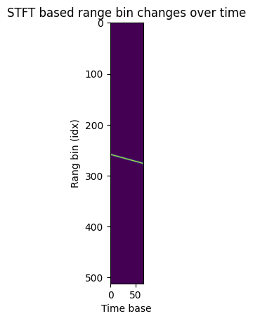
compute speed after STFT

from scipy.signal import find_peaks
# find the range bin where target is at the begining of STFT
peak_at_start = find_peaks(abs(fft_st[:,0]))[0][0]
# find the range bin where the target is at the end of STFT
peak_at_end = find_peaks(abs(fft_st[:,-1]))[0][0]

# speed = Delta D/Delta T

# Range bin resolution from samples
R_bin_fft = fs0*c/2/chirp_slope0/NA
# Range bin resolution for STFT is scaled up by nperseg
R_bin_stft = R_bin_fft*NA/seg_n
# compute the chirp time, which is also the divider for the speed
Tc = NA*1/fs0
# The target distance grows 2x (there and back) so speed needs to be divided by 2
speed_estimate = (peak_at_end-peak_at_start)*R_bin_stft/Tc/2
print(f"speed estimate: {speed_estimate}")

speed estimate: 20599.365234375

non regression

from datetime import datetime as dt
assert speed_estimate==20599.365234375
print(f"last run: {dt.now().date()}")

last run: 2026-06-27