FMCW Intro
You can open this workbook in Google Colab to experiment with mmWrt 
Below is an intro to mmWrt for simple scatterers position estimation
For a generic introduction to mmWave sensors: Watch Here
linear chirps and IF frequencies
Signal model According to (Barriok 1973; Stove 1992; Komarov and Smolskiy 2003; Winkler 2007) the transmitted signal of an FMCW radar system can be modeled as where
Given for a linear chirp that
We derive the phase, given
which can be written as:
Where:
\(f_{0min}\) is the start frequency at the begining of the raising frequency of the chirp.
s is the slope at which the frequency is ramped ( \(S = \frac{B}{T}\))
B is the total bandwdith of the chirp
T is the total time of the chirp
Considering a reflected signal with a time delay \(\delta = 2 · \frac{R0+ v\cdot t}{c}\) and Doppler shift \(f_D = −2 · \frac{f_c \cdot v}{c}\)
Where:
c is the speed of light
\(f_D\) is the doppler shift
R0 is the nominal distance to the target
\(\Delta\) is the time of flight (to and from the target)
v is the velocity of the target
The receive signal \(y_R(t)\) can be written as :
\(y_{IF}(t)\) is the IF signal (after mixer) which is obtained by multiplication in the time domain, and passed to a low-pass filter (LPF)
This can be done easily when remembering the trigonometric relation:
Noticing that the element which sums the elements will be higher frequency and will be filtered by the LPF, it remains that:
Where:
\(f_{0min}\) the starting frequency of the chirp
s is the slope of the chirp
\(\Delta\) is the total time of flight between antennas and target
At, Ar: Amplitude of the RX and TX waves
[8]:
# Install a pip package in the current Jupyter kernel
import sys
from os.path import abspath, basename, join, pardir
import datetime

# hack to handle if running from git cloned folder or stand alone (like Google Colab)
cw = basename(abspath(join(".")))
dp = abspath(join(".",pardir))
if cw=="docs" and basename(dp) == "mmWrt":
    # running from cloned folder
    print("running from git folder, using local path (latest) mmWrt code", dp)
    sys.path.insert(0, dp)
else:
    print("running standalone, need to ensure mmWrt is installed")
    !{sys.executable} -m pip install mmWrt
print(datetime.datetime.now())
running from git folder, using local path (latest) mmWrt code c:\git\mmWrt
2026-07-17 18:51:00.369680
[9]:
from os.path import abspath, join, pardir
import sys
import matplotlib.pyplot as plt
from matplotlib import colormaps
from matplotlib import colors
from numpy import where, expand_dims

from mmWrt.Raytracing import rt_points  # noqa: E402
from mmWrt.Scene import Radar, Transmitter, Receiver, Scatterer  # noqa: E402
from mmWrt import RadarSignalProcessing as rsp  # noqa: E402
from mmWrt import __version__ as mmWrt_version
[10]:
c = 3e8

debug_ON = False
test = 0
chirp_bandwidth = 2e9  # 1e9
chirp_slope0 = 5e12  #280e8
chirp_end_time0 = chirp_bandwidth/chirp_slope0

radar = Radar(transmitter=Transmitter(chirp_end_time=chirp_end_time0,
                                      chirp_slope=chirp_slope0),
              receiver=Receiver(adc_sample_rate=1e6,
                                adc_sample_count=128,
                                debug=debug_ON), debug=debug_ON)

# artificially define scatters so they fall in the
# middle of range bin for illustration purposes
# later of what happen when it is not the case
scatterer1 = Scatterer(5.0390625)
scatterer2 = Scatterer(2*5.0390625)
scatterers = [scatterer1, scatterer2]

bb = rt_points([radar],
               scatterers,
               radar, debug=debug_ON)
Distances, range_profile = rsp.range_fft(bb["adc_cube"][0,0,0,:], bb)
mag_r = abs(range_profile)
ca_cfar = rsp.cfar_ca(mag_r, train_cell_count=10,
                      guard_cell_count=1, pfa=1e-1)
mag_c = abs(ca_cfar)
# little hack to remove small FFT ripples : mag_r> 5
target_filter = ((mag_r > mag_c) & (mag_r > 5))

index_peaks = where(target_filter)[0]
# grouped_peaks = rsp.peak_grouping_1d(index_peaks)

found_scatterers = [Scatterer(Distances[i]) for i in index_peaks]
error = rsp.error([scatterer1, scatterer2], found_scatterers)
print("synthetic scatterers", [t.distance() for t in scatterers])
print("found scatterers", [t.distance() for t in found_scatterers])
print("error is", error)

# 2D representation of the FFT and CFAR
# plot on X,Y axis the FFT and CFAR
plt.plot(Distances, mag_r)
plt.plot(Distances, mag_c)
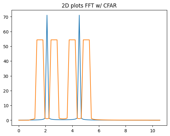
plt.title("2D plots FFT w/ CFAR")
plt.show()
synthetic scatterers [np.float64(5.0390625), np.float64(10.078125)]
found scatterers [np.float64(4.921875), np.float64(5.15625), np.float64(10.078125)]
error is 5.0390625
[11]:
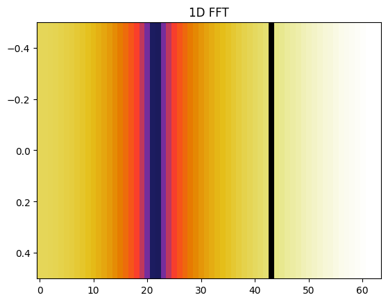
# 1D representation of the FFT
# useful later on to show the link between 1D FFT and 2D FFTs

# Select the color map named CMRmap_r
# cmap = cm.get_cmap(name='CMRmap_r')
cmap = colormaps['CMRmap_r']
# convert the 1D array in 2D array to plot using imshow
mag_r_2d = expand_dims(mag_r, axis=0)
# set aspect ratio to auto to have high enough pixels to see them in the y_axis
# change the norm to have a log color scale
# to better see the peaks in correlation with 2D FFT plot
vmin_mag = min(mag_r)
vmax_mag = max(mag_r)
color_col = colors.LogNorm(vmin=vmin_mag, vmax=vmax_mag)
plt.imshow(mag_r_2d, cmap,
           aspect='auto',
           norm=color_col)
plt.title("1D FFT")
# plt.savefig(fp_fft_1D)
plt.show()
NON REGRESSION
[12]:
from datetime import datetime as dt
assert index_peaks[0]==21
print(f"last run: {dt.now().date()} with {mmWrt_version}")
last run: 2026-07-17 with 0.0.14.dev1+g243a05bf3.d20260717