MIMO TDM
You can open this workbook in Google Colab to experiment with mmWrt 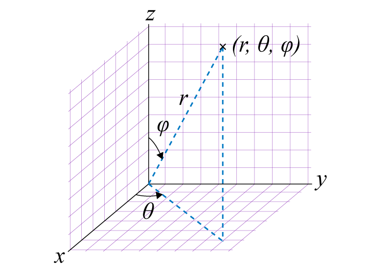
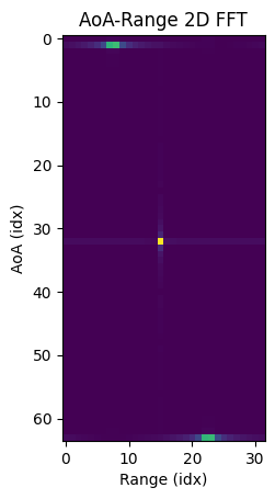
Below is an intro to mmWrt for simple targets position in (X,Y) plane based on 2D FFT (Range, Azimuth) FFTs with a TDM MIMO.
TDM MIMO ULA
Setup
[1]:
# Install a pip package in the current Jupyter kernel
import sys
from os.path import abspath, basename, join, pardir
import datetime

# hack to handle if running from git cloned folder or stand alone (like Google Colab)
cw = basename(abspath(join(".")))
dp = abspath(join(".",pardir))
if cw=="docs" and basename(dp) == "mmWrt":
    # running from cloned folder
    print("running from git folder, using local path (latest) mmWrt code", dp)
    sys.path.insert(0, dp)
else:
    print("running standalone, need to ensure mmWrt is installed")
    !{sys.executable} -m pip install mmWrt

from os.path import abspath, join, pardir
import sys
from numpy.fft import fft, fftshift
from scipy.signal import find_peaks
import matplotlib.pyplot as plt
from numpy import arange, cos, sin, pi, zeros, abs as np_abs

from mmWrt.Scene import Antenna, Medium, Radar, Receiver, Scatterer, Transmitter
from mmWrt.Raytracing import rt_points
from mmWrt import __version__
print("version:", __version__)

print(datetime.datetime.now())
running from git folder, using local path (latest) mmWrt code c:\git\mmWrt
version: 0.0.14.dev1+g243a05bf3.d20260717
2026-07-17 18:56:19.971900
[2]:
f0 = 62e9
# Number of ADC samples
NA = 64
# Number of TX channels
NT = 8
# Number of RX channels
NR = 8
_fs = 4e3
_k = 70e8
chirp_bandwidth0 = 3.5e9

chirp_slope0 = _k
chirp_end_time0 = chirp_bandwidth0 / chirp_slope0
chirp_count0 = NT
chirp_period0 = chirp_end_time0*1.1

adc_sample_rate0 = _fs
adc_sample_count0 = NA

void = Medium()
c = void.v
lambda0 = c/f0
TXs = [Antenna(x=NR*lambda0/2*i) for i in range(NT)]
RXs = [Antenna(x=lambda0/2*i) for i in range(NR)]

radar = Radar(transmitter=Transmitter(chirp_end_time=chirp_end_time0,
                                      chirp_slope=chirp_slope0,
                                      chirp_count=chirp_count0,
                                      chirp_period=chirp_period0,
                                      frame_period=chirp_period0*64,
                                      antennas=TXs),
              receiver=Receiver(adc_sample_rate=adc_sample_rate0,
                                adc_sample_count=adc_sample_count0,
                                adc_sample_count_max=2048,
                                antennas=RXs),
              debug=False)

r1, theta1 = 10.1, 0
x1, y1 = r1*cos(theta1), r1*sin(theta1)
r2, theta2 = 20.1, pi/2
x2, y2 = r2*cos(theta2), r2*sin(theta2)
r3, theta3 = 30.1, pi
x3, y3 = r3*cos(theta3), r3*sin(theta3)

scatterer1 = Scatterer(x1, y1, 0)  # 0 degrees on x-axis <=> -pi/2 vs bore sight
scatterer2 = Scatterer(x2, y2, 0) # pi/2 degrees vs x-ax <=> 0 degree vs bore sight
scatterer3 = Scatterer(x3, y3, 0) # 180 degrees on x-axis <=> pi/2 vs boresight
scatterers = [scatterer1, scatterer2, scatterer3]

bb = rt_points([radar],
               scatterers,
               radar,
               debug=False)
cube = bb["adc_cube"][0,:,:,:]

virtual_cube = zeros((NR*NT, NA))
# cube.reshape((NR*NT, NA)) is
# equivalent to:
# for chirp_idx in range(chirp_count0):
#    for rx_idx in range(NR):
#        virtual_cube[chirp_idx*NR+rx_idx,:] = cube[chirp_idx, rx_idx, :]

virtual_cube = cube.reshape((NR*NT, NA))

fast_time_axis = 1
virtual_antennas_axis = 0
# first compute the range FFT
R_fft = fft(virtual_cube, axis=fast_time_axis)
# then compute the AoA FFT
A_FFT = fft(R_fft, axis=virtual_antennas_axis)

# for Range vs AoA, display magnitude
# and need to fftshift to have the negative frequencies moved around 0
Z_fft = abs(fftshift(A_FFT[:,:], axes=0))
plt.xlabel("Range (idx)")
plt.ylabel("AoA (idx)")
plt.title('AoA-Range 2D FFT')
# plt.plot(np_abs(np.sum(R_fft, axis=0)))
plt.imshow(Z_fft[:,:NA//2])
plt.show()
ULA in elevation
[3]:
## ULA in elevation
NT = 7
# Number of RX channels
NR = 7

# Now define target1 with an elevation:
r1, theta1, phi1 = 10.1, pi/2, pi*0.0
x1 = r1 * cos(theta1)*sin(phi1)
y1 = r1 * sin(theta1)*sin(phi1)
z1 = r1 * cos(phi1)

r2, theta2, phi2 = 20.1, pi/2, pi/2
x2 = r2 * sin(phi2)*cos(theta2)
y2 = r2 * sin(phi2)*sin(theta2)
z2 = r2 * cos(phi2)

r3, theta3, phi3 = 30.1, pi/2, pi*0.99
x3 = r3 * sin(phi3)*cos(theta3)
y3 = r3 * sin(phi3)*sin(theta3)
z3 = r3 * cos(phi3)
scatterer1 = Scatterer(x1, y1, z1)  # 0 degrees on x-axis <=> -pi/2 vs bore sight
scatterer2 = Scatterer(x2, y2, z2) # pi/2 degrees vs x-ax <=> 0 degree vs bore sight
scatterer3 = Scatterer(x3, y3, z3) # 180 degrees on x-axis <=> pi/2 vs boresight

# offset so that middle antenna is at 0,0,0
TXs = [Antenna(y=NR*lambda0/2*i - (NR*lambda0/2)) for i in range(NT)]
RXs = [Antenna(y=lambda0/2*i - ((NR-1)//2)*lambda0/2) for i in range(NR)]

radar = Radar(transmitter=Transmitter(chirp_end_time=chirp_end_time0,
                                      chirp_slope=chirp_slope0,
                                      chirp_count=NT,
                                      chirp_period=chirp_period0,
                                      frame_period=chirp_period0*64,
                                      antennas=TXs),
              receiver=Receiver(adc_sample_rate=adc_sample_rate0,
                                adc_sample_count=adc_sample_count0,
                                adc_sample_count_max=2048,
                                antennas=RXs),
              debug=False)

scatterers = [scatterer1, scatterer2, scatterer3]
print([f"{s}" for s in scatterers])
bb = rt_points([radar], scatterers,
               radar,
               debug=False)
cube = bb["adc_cube"][0,:,:,:]

# generate virtual antennas
virtual_cube = cube.reshape(( NT * NR, NA))

RX_antennas_axis = 0
fast_time_axis = 1
# first compute the range FFT
R_fft = fft(virtual_cube, axis=fast_time_axis)
# then compute the AoA FFT
A_FFT = fft(R_fft, axis=RX_antennas_axis)

# for Range vs AoA, display magnitude
# and need to fftshift to have the negative frequencies moved around 0
Z_fft = abs((A_FFT[:,:]))
plt.xlabel("Range (idx)")
plt.ylabel("AoA (idx)")
plt.title('AoA-Range 2D FFT')
plt.imshow(Z_fft[:,:NA//2])
plt.show()
['x0:0.0, y0:0.0, z0:10.1', 'x0:1.2307700331430901e-15, y0:20.1, z0:1.2307700331430901e-15', 'x0:5.789296377354671e-17, y0:0.94546384825166, z0:-30.08514746700852']
URA
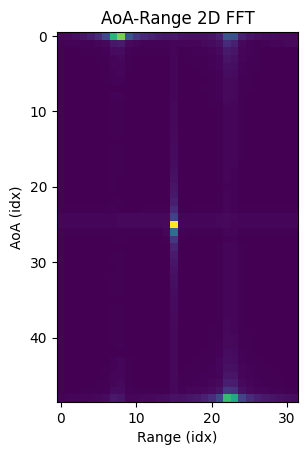
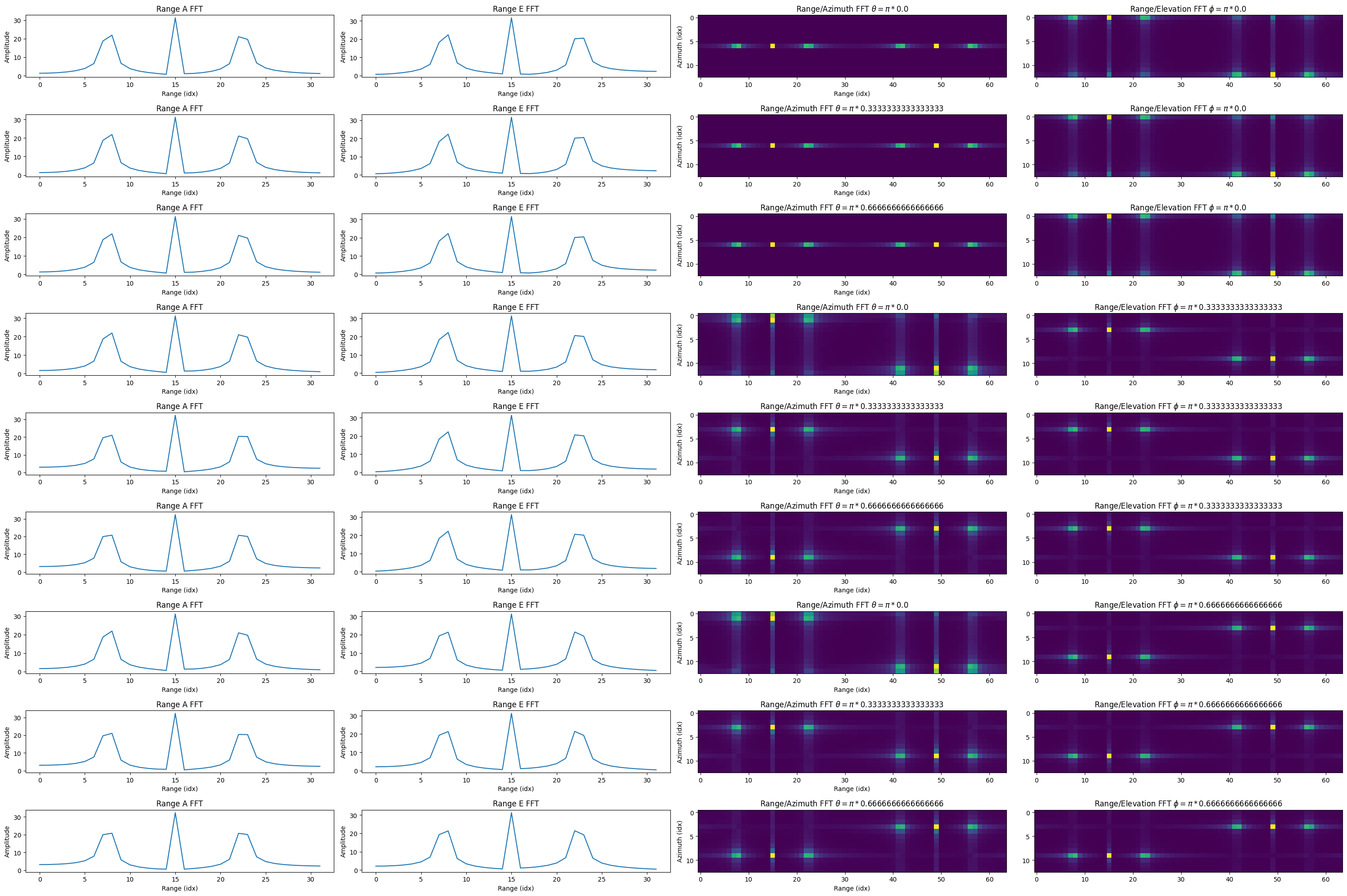
We are now considering the case where the targets have an elevation (i.e. a z dimension not null).
(r, \(\theta\), \(\phi\)) are defined as per polar coordinates:
$ x = r * \sin`(:nbsphinx-math:phi`) \cdot `:nbsphinx-math:cos`(\theta) $
$ y = r * \sin`(:nbsphinx-math:phi`) \cdot `:nbsphinx-math:sin`(\theta) $
$ z = r * \cos`(:nbsphinx-math:phi`) $
[4]:
# first redefine the TX antennas:
# instead of TX being NR*lambda0/2 apart on the x-axis to have a ULA,
# we define them lambda0/2 on the y-axis to have a URA
NT = 13
NR = 13
TXs = [Antenna(z=lambda0/2*i - ((NT-1)//2)*lambda0/2) for i in range(NT)]
RXs = [Antenna(x=lambda0/2*i - ((NR-1)//2)*lambda0/2) for i in range(NR)]
# then update the radar definition
chirp_bandwidth0 = 3.5e9
chirp_slope0 = _k
chirp_end_time0 = chirp_bandwidth0/chirp_slope0
adc_sample_rate0=_fs
adc_sample_count0=NA
chirp_period0 = NA*chirp_end_time0*1.1
frame_period0 = NT*chirp_period0*1.1
radar = Radar(transmitter=Transmitter(chirp_end_time=chirp_end_time0,
                                      chirp_slope=chirp_slope0,
                                      chirp_count=NT,
                                      chirp_period=chirp_period0,
                                      frame_period=frame_period0,
                                      antennas=TXs),
              receiver=Receiver(adc_sample_rate=adc_sample_rate0,
                                adc_sample_count_max=2048,
                                adc_sample_count=adc_sample_count0,
                                antennas=RXs),
              debug=False)

# Now define target1 with an elevation:
theta, phi = pi*0.0, pi*1.0
theta_steps = 3
phi_steps = 3
fig, axs = plt.subplots(ncols=4, nrows=theta_steps*phi_steps, figsize=(30,20))

for phi_idx in range(phi_steps):
    for theta_idx in range(theta_steps):
        theta0, phi0 = theta_idx/theta_steps, phi_idx/phi_steps
        theta, phi = theta0*pi, phi0*pi
        r1, theta1, phi1 = 10.1, theta, phi
        x1 = r1 * cos(theta1)*sin(phi1)
        y1 = r1 * sin(theta1)*sin(phi1)
        z1 = r1 * cos(phi1)
        r2, theta2, phi2 = 20.1, theta, phi
        x2 = r2 * cos(theta2)*sin(phi2)
        y2 = r2 * sin(theta2)*sin(phi2)
        z2 = r2 * cos(phi2)
        r3, theta3, phi3 = 30.1, theta, phi
        x3 = r3 * sin(phi3)*cos(theta3)
        y3 = r3 * sin(phi3)*sin(theta3)
        z3 = r3 * cos(phi3)
        scatterer1 = Scatterer(x1, y1, z1)
        scatterer2 = Scatterer(x2, y2, z2)
        scatterer3 = Scatterer(x3, y3, z3)
        scatterers = [scatterer1, scatterer2, scatterer3]

        bb = rt_points([radar],
                       scatterers,
                       radar,
                       debug=False)
        cube = bb["adc_cube"][0,:,:,:]

        # define virtual cubes
        virtual_cube_azimuth = zeros(( NR, NA)).astype(complex)
        virtual_cube_elevation = zeros(( NT , NA)).astype(complex)
        for rx_idx in range(NR):
            virtual_cube_azimuth[rx_idx,:] = cube[(NT-1)//2, rx_idx, :]
        for tx_idx in range(NT):
            virtual_cube_elevation[tx_idx,:] = cube[tx_idx, (NR-1)//2, :]

        # compute (just to show this is the same
        # Range FFT from Azi and Ele cubes
        RF1 = fft(virtual_cube_azimuth, axis=-1)
        RF2 = fft(virtual_cube_elevation, axis=-1)

        # Range Azimuth cube
        RA = fftshift(fft(RF1, axis=0), axes=0)
        # Range Elevation cube
        RE = fftshift(fft(RF2, axis=0), axes=0)

        ax0, ax1, ax2, ax3 = axs[theta_idx+(theta_steps)*phi_idx, 0], axs[theta_idx+(theta_steps)*phi_idx, 1], \
            axs[theta_idx+(theta_steps)*phi_idx,2],axs[theta_idx+(theta_steps)*phi_idx, 3]

        # show Range FFT from Azi FFT
        ax0.set_xlabel("Range (idx)")
        ax0.set_ylabel("Amplitude")
        ax0.set_title('Range A FFT')
        ax0.plot(abs(RF1[0,:NA//2]))

        # show Range FFT from Ele FFT
        ax1.set_xlabel("Range (idx)")
        ax1.set_ylabel("Amplitude")
        ax1.set_title('Range E FFT')
        ax1.plot(abs(RF2[0,:NA//2]))

        # Show Range Azi map
        ax2.set_xlabel("Range (idx)")
        ax2.set_ylabel("Azimuth (idx)")
        ax2.set_title(fr'Range/Azimuth FFT $\theta = \pi *{theta0}$')
        # use interpolation and aspect to have the map same size as Range FFT
        ax2.imshow(abs(RA), interpolation='nearest', aspect='auto')

        # Show Range Ele map
        ax3.set_title(f"Range/Elevation FFT $\phi= \pi *{phi0}$")
        # use interpolation and aspect to have the map same size as Range FFT
        ax3.imshow(abs(RE),interpolation='nearest', aspect='auto')
plt.tight_layout()
[5]:
# first redefine the TX antennas:
# instead of TX being NR*lambda0/2 apart on the x-axis to have a ULA,
# we define them lambda0/2 on the y-axis to have a URA
NT = 13
NR = 13
TXs = [Antenna(z=lambda0/2*i - ((NT-1)//2)*lambda0/2) for i in range(NT)]
RXs = [Antenna(x=lambda0/2*i - ((NR-1)//2)*lambda0/2) for i in range(NR)]
# then update the radar definition
chirp_bandwidth0 = 3.5e9
chirp_slope0 = _k
chirp_end_time0 = chirp_bandwidth0/chirp_slope0
adc_sample_rate0 = _fs
adc_sample_count0 = NA
chirp_period0 = chirp_end_time0*1.1
frame_period0 = NT*chirp_period0*1.1
radar = Radar(transmitter=Transmitter(chirp_end_time=chirp_end_time0,
                                      chirp_slope=chirp_slope0,
                                      chirp_count=NT,
                                      chirp_period=chirp_period0,
                                      frame_period=frame_period0,
                                      antennas=TXs),
              receiver=Receiver(adc_sample_rate=adc_sample_rate0,
                                adc_sample_count_max=2048,
                                adc_sample_count=adc_sample_count0,
                                antennas=RXs),
              debug=False)

# Now define target1 with an elevation:

r1, theta1, phi1 = 10.1, 0, pi/2
x1 = r1 * cos(theta1)*sin(phi1)
y1 = r1 * sin(theta1)*sin(phi1)
z1 = r1 * cos(phi1)
r2, theta2, phi2 = 20.1, pi/2, pi/2
x2 = r2 * cos(theta2)*sin(phi2)
y2 = r2 * sin(theta2)*sin(phi2)
z2 = r2 * cos(phi2)
r3, theta3, phi3 = 30.1, pi/2, 0
x3 = r3 * sin(phi3)*cos(theta3)
y3 = r3 * sin(phi3)*sin(theta3)
z3 = r3 * cos(phi3)
scatterer1 = Scatterer(x1, y1, z1)
scatterer2 = Scatterer(x2, y2, z2)
scatterer3 = Scatterer(x3, y3, z3)
scatterers = [scatterer1, scatterer2, scatterer3]
print("scatterers", [f"{s}" for s in scatterers])

bb = rt_points([radar],
               scatterers,
               radar,
               debug=False)
cube = bb["adc_cube"]

range_azimuth_fft = fftshift(fft(fft(cube[0,0,:NR,:], axis=-1), axis=-2), axes=-2)

fig, (ax0) = plt.subplots(ncols=1)
# ax0.imshow(abs(RA[(NT-1)//2,:,:NA//2]))
ax0.imshow(np_abs(range_azimuth_fft[:,:NA//2]))
ax0.set_title("Range Azimuth map")
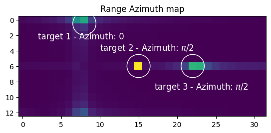
azi_target1 = plt.Circle((8, 0.5), 1.5, fill=False, color="white")
azi_target2 = plt.Circle((15, 6), 1.5, fill=False, color="white")
azi_target3 = plt.Circle((22, 6), 1.5, fill=False, color="white")
ax0.text(2, 2.5, f"target 1 - Azimuth: 0", color="white", fontsize=12)
ax0.text(10, 4, f"target 2 - Azimuth: $\pi$/2", color="white", fontsize=12)
ax0.text(17, 9, f"target 3 - Azimuth: $\pi$/2", color="white", fontsize=12)
ax0.add_artist(azi_target1)
ax0.add_artist(azi_target2)
ax0.add_artist(azi_target3)
plt.show()
scatterers ['x0:10.1, y0:0.0, z0:6.184466335694133e-16', 'x0:1.2307700331430901e-15, y0:20.1, z0:1.2307700331430901e-15', 'x0:0.0, y0:0.0, z0:30.1']
[6]:
range_elevation_fft = fftshift(fft(fft(cube[0,:,0,:], axis=-1), axis=0), axes=0)

fig, (ax0) = plt.subplots(ncols=1)
ax0.imshow(abs(range_elevation_fft[:,:NA//2]))
ax0.set_title("Range Elevation map")
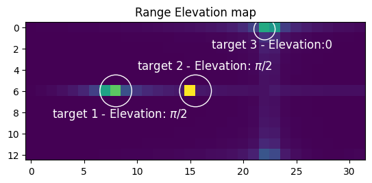
ele_target1 = plt.Circle((8, 6), 1.5, fill=False, color="white")
ele_target2 = plt.Circle((15.5, 6), 1.5, fill=False, color="white")
ele_target3 = plt.Circle((22, 0.2), 1, fill=False, color="white")
ax0.text(2, 8.5, f"target 1 - Elevation: $\pi$/2", color="white", fontsize=12)
ax0.text(10, 4, f"target 2 - Elevation: $\pi$/2", color="white", fontsize=12)
ax0.text(17, 2, f"target 3 - Elevation:0", color="white", fontsize=12)
ax0.add_artist(ele_target1)
ax0.add_artist(ele_target2)
ax0.add_artist(ele_target3)
[6]:
<matplotlib.patches.Circle at 0x28ed7873a00>
[18]:
from mmWrt.RadarSignalProcessing import cfar_ca, if2d
from numpy import where, concatenate, abs
def pcl(cube):
    Range_FFT = fft(cube, axis=-1)
    range0 = Range_FFT[0,0,0,:NA//2]

    # cfar_th = cfar_1d(range0, num_training_cells=8, mode="full", cfar_type="CA")
    cfar_th = cfar_ca(abs(range0), train_cell_count=8,
                      guard_cell_count=1, pfa=1e-1)
    target_filter = ((abs(range0) > abs(cfar_th)) & (abs(range0) > 20))
    index_peaks = where(target_filter)
    # focus on range bins where some targets are detected
    # lowers memory constraints for follow-up FFTs
    # usually the highest return as the fast time dimension is usually the largest
    range_targets = Range_FFT[:,:,:,index_peaks[0]]
    azi_FFT = fft(range_targets, axis=-2)
    ele_FFT = fft(azi_FFT, axis=-3)
    scatterers = []
    for range_idx in range(len(index_peaks[0])):
        target0_azi = azi_FFT[0,0,:,range_idx]
        cfar_th_a = cfar_ca(abs(target0_azi),
                            train_cell_count=4,
                            guard_cell_count=1, pfa=1e-1)  #, mode="full", debug=False, cfar_type="CA")
        target_filter = ((abs(target0_azi) > abs(cfar_th_a)))
        index_peaks_azi = where(target_filter)[0]
        mag_azis = abs(azi_FFT[0,0,index_peaks_azi,range_idx])
        # simplification: here we only look for one peak
        # FIXME: should do peak grouping here to retrieve all targets
        # the alternative to take all peaks from CFAR just yields too many targets
        azi_idxs = [[m for m in mag_azis].index(max(mag_azis))]
        for azi_idx in azi_idxs:
            target0_ele = ele_FFT[0,:,index_peaks_azi[azi_idx],range_idx]
            cfar_th_e = cfar_ca(abs(target0_ele), train_cell_count=4,guard_cell_count=1,
                                pfa=1e-1)
            #                    mode="full", debug=False, cfar_type="CA")
            target_filter = ((abs(target0_ele) > abs(cfar_th_e)))
            index_peaks_ele = where(target_filter)[0]
            mag_eles = abs(ele_FFT[0,index_peaks_ele,azi_idx,range_idx])
            # same comment as for azimuth: here should do peak grouping
            # today only grabs the strongest echo in elevation
            e_idx = [m for m in mag_eles].index(max(mag_eles))
            scatterers.append((index_peaks[0][range_idx], index_peaks_azi[azi_idx], index_peaks_ele[e_idx]))
    return scatterers

print("cube shape",cube.shape)
scatterer_detected = pcl(cube)
print("scatterer_detected", scatterer_detected)
f2d = if2d(radar)
scatterer_range = [(f_idx*_fs*f2d/NA, a, e) for f_idx, a, e in scatterer_detected]
print("scatterer_range", scatterer_range)
cube shape (1, 13, 13, 64)
scatterer_detected [(np.int64(8), np.int64(7), np.int64(0)), (np.int64(15), np.int64(0), np.int64(0)), (np.int64(22), np.int64(0), np.int64(7)), (np.int64(23), np.int64(0), np.int64(7))]
scatterer_range [(np.float64(10.714285714285714), np.int64(7), np.int64(0)), (np.float64(20.089285714285715), np.int64(0), np.int64(0)), (np.float64(29.464285714285715), np.int64(0), np.int64(7)), (np.float64(30.80357142857143), np.int64(0), np.int64(7))]
[20]:
def AoA_idx_to_rad(phi_idx, tot=13):
    from numpy import arcsin
    if phi_idx<tot/2:
        arg_phi = phi_idx/(tot/2)
    else:
        arg_phi = phi_idx-tot
        arg_phi /= tot/2
    phi = pi/2 + arcsin(arg_phi)
    return phi
def pol2cart(p):
    r, theta, phi = p
    print("r, t, p", r, theta, phi)
    x = r * cos(theta)*sin(phi)
    y = r * sin(theta)*sin(phi)
    print("y", y)
    z = r * cos(phi)
    return (x,y,z)
print("scatterer_detected idx", scatterer_detected)
scatterer_polar = [(f_idx*_fs*f2d/NA, AoA_idx_to_rad(a), AoA_idx_to_rad(e)) for f_idx, a, e in scatterer_detected]
print("scatterer_polar", scatterer_polar)
scatterer_cartesian = [pol2cart(p) for p in scatterer_polar]
print("target cartesians", scatterer_cartesian)
scatterer_detected idx [(np.int64(8), np.int64(7), np.int64(0)), (np.int64(15), np.int64(0), np.int64(0)), (np.int64(22), np.int64(0), np.int64(7)), (np.int64(23), np.int64(0), np.int64(7))]
scatterer_polar [(np.float64(10.714285714285714), np.float64(0.39479111969976133), np.float64(1.5707963267948966)), (np.float64(20.089285714285715), np.float64(1.5707963267948966), np.float64(1.5707963267948966)), (np.float64(29.464285714285715), np.float64(1.5707963267948966), np.float64(0.39479111969976133)), (np.float64(30.80357142857143), np.float64(1.5707963267948966), np.float64(0.39479111969976133))]
r, t, p 10.714285714285714 0.39479111969976133 1.5707963267948966
y 4.120879120879119
r, t, p 20.089285714285715 1.5707963267948966 1.5707963267948966
y 20.089285714285715
r, t, p 29.464285714285715 1.5707963267948966 0.39479111969976133
y 11.332417582417577
r, t, p 30.80357142857143 1.5707963267948966 0.39479111969976133
y 11.847527472527467
target cartesians [(np.float64(9.89010989010989), np.float64(4.120879120879119), np.float64(6.560607852575106e-16)), (np.float64(1.2301139723578325e-15), np.float64(20.089285714285715), np.float64(1.2301139723578325e-15)), (np.float64(6.939104459454436e-16), np.float64(11.332417582417577), np.float64(27.1978021978022)), (np.float64(7.254518298520547e-16), np.float64(11.847527472527467), np.float64(28.434065934065938))]
[ ]: