FMCW-Radar-107_Micro-Doppler
You can open this workbook in Google Colab to experiment with mmWrt ![]()
Below is an intro to mmWrt for simple micro doppler estimation
[1]:
# Install a pip package in the current Jupyter kernel
import sys
from os.path import abspath, basename, join, pardir
import datetime

# hack to handle if running from git cloned folder or stand alone (like Google Colab)
cw = basename(abspath(join(".")))
dp = abspath(join(".",pardir))
if cw=="docs" and basename(dp) == "mmWrt":
    # running from cloned folder
    print("running from git folder, using local path (latest) mmWrt code", dp)
    sys.path.insert(0, dp)
else:
    print("running standalone, need to ensure mmWrt is installed")
    !{sys.executable} -m pip install mmWrt
print(datetime.datetime.now())
running from git folder, using local path (latest) mmWrt code c:\git\mmWrt
2026-06-23 20:57:19.606285
[25]:
from os.path import abspath, join, pardir
import sys
from numpy import arange, array, expand_dims, pi, sin, where, zeros
from numpy import complex128 as complex
from numpy.fft import fft, fftshift, fft2, fftshift, fftfreq
from scipy.signal import find_peaks, stft

import matplotlib.pyplot as plt
from numpy import arange, cos, sin, pi, zeros
import numpy as np

from mmWrt.Scene import Antenna, Medium
from mmWrt.Raytracing import rt_points  # noqa: E402
from mmWrt.Scene import Radar, Transmitter, Receiver, Scatterer  # noqa: E402
from mmWrt import RadarSignalProcessing as rsp  # noqa: E402

from mmWrt.Raytracing import rt_points
from mmWrt import __version__ as mmWrt_ver
print(mmWrt_ver)

print("last run on ", datetime.datetime.now())
0.0.11-pre.3
last run on  2026-06-23 21:14:18.861178
[4]:
import matplotlib.pyplot as plt
import matplotlib.cm as cm
from matplotlib import colors
[53]:
opt = {"compute":True, "Dres_min":50, "BW":0.01e9, "k":15e12, "NC":32, "NA":64,  "fs":100e6, "f0_min":60e9, "NF":256,
        "d0": 50, "v0": 160,
        "TIC":1.2e-6, "TIF": 1.2e-3,
        "logger": "TBD",
        "xt1": "lambda t: d0 + t*v0", "xt": "lambda t: 4*A0*sin(2*pi*f1*t)+d0"}

d0, v0 = opt["d0"], opt["v0"]
NC = opt["NC"]
NA = opt["NA"]
NF = opt["NF"]
BW = opt["BW"]
k = opt["k"]
fs = opt["fs"]
f0_min=opt["f0_min"]
TIF = opt["TIF"]
TIC = opt["TIC"]
F1 = 6
f1 = F1/(NF*TIF)
A0 = v0/(2*pi*f1)
udops1 = zeros((NC, NF))

xt = eval(opt["xt"])

chirp_slope0 = k
chirp_end_time0 = BW/chirp_slope0

adc_sample_rate0 = fs

radar = Radar(transmitter=Transmitter(chirp_end_time=chirp_end_time0,
                                      chirp_slope=chirp_slope0,
                                      chirp_start_freq=f0_min,
                                      chirp_period=TIC,
                                      frame_period=TIF,
                                      frame_count=NF,
                                      chirp_count=NC),
              receiver=Receiver(adc_sample_rate=adc_sample_rate0,
                                adc_sample_count_max=1024,
                                adc_sample_rate_max=110e6,
                                adc_sample_count = NA),
             debug=False)


target = Scatterer(xt=lambda t: xt(t))

bb = rt_points([radar], [target],
               radar,
               datatype=complex, raytracing_opt=opt,
               debug=False)

cube0 = bb["adc_cube"][0,0,0,:]
6.666666666666667e-07 1e-08 1.6666666666666668e-07
[57]:
rx_i = 0

for frame_idx in range(NF):
    # compute range doppler
    cube = bb["adc_cube"][frame_idx,:,rx_i,:]
    Z_fft2 = abs(fftshift(fft2(cube)))
    # find peak in range
    pk0 = find_peaks(abs(fft(cube[0,:])))[0][0]
    pk1 = find_peaks(abs(fft(cube[-1,:])))[0][0]
    # non regression hook
    assert pk0 == pk1
    # append doppler bin at peak range
    udops1[:,frame_idx] = Z_fft2[:, pk0]
dop_idx = find_peaks(abs(Z_fft2[:, pk0]))[0][0]
# non regression hook
assert dop_idx == 26

plt.figure(figsize=(10,6))
fig, [ax0, ax1] = plt.subplots(nrows=2)
ax0.imshow(abs(Z_fft2))
ax0.set_title(f"Range-Doppler for frame: {frame_idx}")
ax0.set_xlabel("Range idx")
ax0.set_ylabel("Dop idx")
ax1.set_title("single target")
ax1.imshow(udops1, aspect='auto')
plt.tight_layout()
<Figure size 1000x600 with 0 Axes>
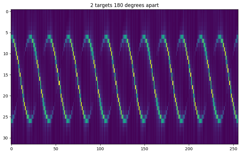
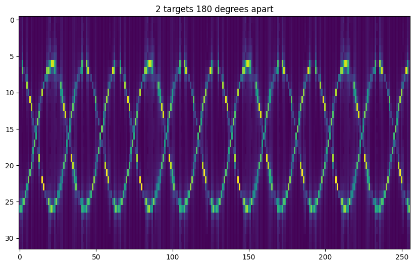
2 Targets 180 degrees
[63]:
# add a scatterer 180 degrees from previous one
scatterer_180 = Scatterer(xt=lambda t: xt(t+1/2*1/f1))
bb = rt_points([radar], [target, scatterer_180],
               radar, datatype=complex,
               raytracing_opt=opt)

udops = zeros((NC, NF))
pk0 = None
tx_i, rx_i = 0, 0

for frame_idx in range(NF):
    # compute range doppler
    cube = bb["adc_cube"][frame_idx,:,rx_i,:]
    Z_fft2 = abs(fftshift(fft2(cube)))
    # find peak in range
    pk = find_peaks(abs(fft(cube[0,:])))[0][0]
    # append doppler bin at peak range
    udops[:,frame_idx] = Z_fft2[:, pk]
plt.figure(figsize=(10,6))
plt.title("2 targets 180 degrees apart")
plt.imshow(udops, aspect='auto')
plt.show()
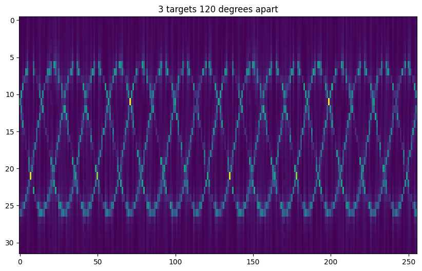
3 Targets each 120 degrees
[62]:
scatterer_120 = Scatterer(xt=lambda t: xt(t+1/3*1/f1))
scatterer_240 = Scatterer(xt=lambda t: xt(t+2/3*1/f1))
bb = rt_points([radar], [target, scatterer_120, scatterer_240],
               radar,
               datatype=complex, raytracing_opt=opt)

udops = zeros((NC, NF))
pk0 = None
tx_i, rx_i = 0, 0

for frame_idx in range(NF):
    # compute range doppler
    cube = bb["adc_cube"][frame_idx,:,rx_i,:]
    Z_fft2 = abs(fftshift(fft2(cube)))
    # find peak in range
    pk = find_peaks(abs(fft(cube[0,:])))[0][0]
    # append doppler bin at peak range
    udops[:,frame_idx] = Z_fft2[:, pk]
plt.figure(figsize=(10,6))
plt.title("3 targets 120 degrees apart")
plt.imshow(udops, aspect='auto')
plt.show()
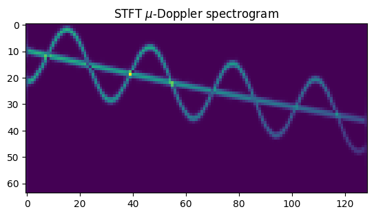
UDOP w/ STFT
STFT can be used to compute \(\mu\)-Doppler when there is only one frame available.
Below also shows when one target has just a linear speed and second target is oscillating around the first one.
[70]:
from scipy.fft import fft, fft2
from numpy import angle, cos, real
from scipy.signal import find_peaks
from scipy.signal import stft

opt = {"compute":True, "Dres_min":50}
debug_ON = False

# chirp start freq
f0m = 60e9
# chirp bandwidth
bw = 1e6
# chirp slope
k=800e6
# t_inter_chirp
t_ic = 2e-3 # 1/2e5
# chirp count
NC=4096
# sampling frequency
fs_if = 21e4
x0, y0, z0 = 500, 0, 500

chirp_end_time0 = bw/k

radar = Radar(transmitter=Transmitter(chirp_end_time=chirp_end_time0,
                                      chirp_slope=k,
                                      chirp_start_freq=f0m,
                                      chirp_period=t_ic,
                                      chirp_count=NC),
              receiver=Receiver(adc_sample_rate=fs_if,
                                adc_sample_count=256,
                                adc_sample_count_max=60000,
                                debug=debug_ON),
              debug=debug_ON)

xt0 = lambda t: v0*t
xt1 = lambda t: xt0(t) + 1*sin(2*pi*f1*t)

# Targets position and speed
xt0 = lambda t: x0+10*t
# 3 rps
f1 = 0.5
xt1 = lambda t: xt0(t) + 0.1*sin(2*pi*f1*t)
scatterer0 = Scatterer(x0, 0, z0, xt=lambda t: xt0(t))
scatterer1 = Scatterer(x0, 0, z0, xt=lambda t: xt1(t))

bb = rt_points([radar], [scatterer0, scatterer1],
               radar,
               datatype=complex, raytracing_opt=opt)
# take the first frame (since only one anyway)
cube = bb["adc_cube"][0, :, 0, :]
# find the range bin where targets are
range_fft = fft(cube)
peaks, _ = find_peaks(abs(range_fft[0]))  # , height=8)

p0 = peaks[0]
range_bin = range_fft[:,p0]
seg_n = NC//64
_,_,B = stft(range_bin, nperseg=seg_n, return_onesided=False)
C = abs(fftshift(B, axes=0))
C = C[:,]
plt.title("STFT $\mu$-Doppler spectrogram")
plt.imshow(C[:,:])
plt.show()
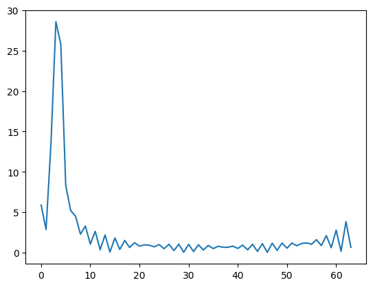
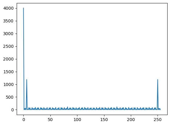
Retrieve oscillation data from uDOP
Simples logic: get the doppler peak location, get the FFT index of those and compare to the setting used to create micro-doppler
[75]:
NC1, NF1 = udops1.shape
dops = []
for frame_idx in range(NF1):
    dop = find_peaks(udops1[:, frame_idx])[0][0]
    dops.append(dop)
Y = fft(dops)
plt.plot(np.abs(Y))
plt.show()
ym = find_peaks(Y)[0][0]
# non regression hook:
# verify that the frequency measured is the same
# as setup at beginning of simulation
# broken during 0.0.11-rc2
assert ym == F1
---------------------------------------------------------------------------
AssertionError                            Traceback (most recent call last)
Cell In[75], line 14
      9 ym = find_peaks(Y)[0][0]
     10 # non regression hook:
     11 # verify that the frequency measured is the same
     12 # as setup at beginning of simulation
     13 # broken during 0.0.11-rc2
---> 14 assert ym == F1

AssertionError:
[ ]:
print("last successful run on ")
print(datetime.datetime.now())
print(mmWrt_ver)
last successful run on
2024-10-27 16:13:46.384196